Principal Component Analysis vs Linear Discriminant Analysis

In machine learning, reducing dimensionality is a critical approach. Overfitting of the learning model may result in a large number of features available in the dataset. There are two standard dimensionality reduction techniques used by machine learning experts to evaluate the collection of essential features and decrease the dataset’s dimension. Dimensionality Reduction in Machine Learning and Statistics reduces the number of random variables under consideration by acquiring a collection of critical variables. It can be divided into feature discovery and extraction of features.
The functional implementation of these two-dimensionality reduction techniques will be discussed in this article.

Principal Component Analysis (PCA)
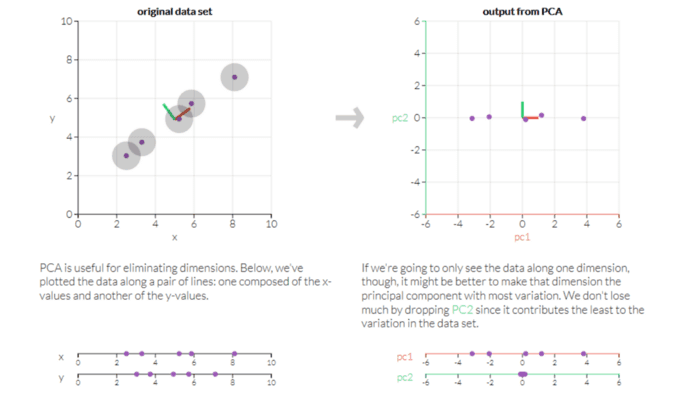
PCA is a technique in unsupervised machine learning that is used to minimize dimensionality. The key idea of the vital component analysis ( PCA) is to minimize the dimensionality of a data set consisting of several variables, either firmly or lightly, associated with each other while preserving to the maximum degree the variance present in the dataset.
This is achieved by translating the variables into a new collection of variables that are a mixture of our original dataset’s variables or attributes so that maximum variance is preserved. This attribute combination is known as Principal Components ( PCs), and the Dominant Principal Component is called the component that has the most variance captured. The order of variance retention decreases as we step down in order, i.e. PC1 > PC2 > PC3 > … and so forth.

Why do we use PCA?
Practically PCA is used for two reasons:
- Dimensionality Reduction: Information spread over many columns is converted into main components ( PCs) such that the first few PCs can clarify a substantial chunk of the total information (variance). In Machine Learning models, these PCs can be used as explanatory variables.
- Visualize classes: It is difficult for data with more than three dimensions (features) to visualize the separation of classes (or clusters). With the first two PCs alone, a simple distinction can generally be observed.
Linear Discriminant Analysis (LDA)
LDA is a technique of supervised machine learning which is used by certified machine learning experts to distinguish two classes/groups. The critical principle of linear discriminant analysis ( LDA) is to optimize the separability between the two classes to identify them in the best way we can determine. LDA is similar to PCA, which helps minimize dimensionality. Still, by constructing a new linear axis and projecting the data points on that axis, it optimizes the separability between established categories.
LDA does not function on finding the primary variable; it merely looks at what kind of point/features/subspace to distinguish the data offers further discrimination.
How are LDA models represented?
The depiction of the LDA is obvious. The model consists of the estimated statistical characteristics of your data for each class. In the case of multiple variables, the same properties are computed over the multivariate Gaussian. The multivariates are matrices of means and covariates. By providing the statistical properties in the LDA equation, predictions are made. From your data, the properties are estimated. Finally, to construct the LDA model, the model values are stored as a file.
LDA Real-Life Applications
Some of the practical LDA applications are described below:
- Face Recognition-In face recognition, LDA is used to reduce the number of attributes until the actual classification to a more manageable number. A linear combination of pixels that forms a template is the dimensions that are created. Fisher’s faces are called these.
- Medical-LDA may be used to identify the illness of the patient as mild, moderate, or extreme. The classification is carried out on the patient’s different criteria and his medical trajectory.
- Customer Identification– By conducting a simple question and answering a survey, you can obtain customers’ characteristics. LDA helps to recognize and pick the assets of a group of consumers most likely to purchase a specific item in a shopping mall.
PCA and LDA Similarities:
- Both list the current axes in order of significance.
- PC1 (the first new axis generated by PCA) accounts for the most significant data variance, PC2 (the second new axis) does the second-best job, and so on …
- LD1 (the first new axis generated by LDA) accounts for the most significant data variance, LD2 (the second new axis) does the second-best job, and so on …
- The algorithms both tell us which attribute or function contributes more to the development of the new axes.
- LDA is like PCA, each attempting to decrease the measurements.
- For the most variation, PCA searches for attributes.
- LDA seeks to optimize the differentiation of groups that are identified.
Conclusion
When we have a linear question in hand, the PCA and LDA are implemented in dimensionality reduction, which means a linear relationship between input and output variables. But it is possible to apply the PCA and LDA together and see the difference in their outcome. While PCA and LDA work on linear issues, they do have differences. The disparity between the data groups is modeled by the LDA, while the PCA does not detect such a disparity between groups. The factor analysis in PCA constructs the combinations of features based on disparities rather than similarities in LDA. As in LDA, the discriminant analysis is different from the factor analysis conducted in PCA where eigenvalues, eigenvectors, and covariance matrices are used. There applications are vast and still being explored by machine learning experts
Related Articles
View All
Machine Learning
Machine Learning Certifications and Career Paths in 2026: Skills, Roles, and Salary Trends
Explore machine learning certifications and career paths in 2026, including in-demand skills, generative AI roles, and salary trends. Learn how to select certifications that map to real deployment work.

Machine Learning
Top Machine Learning Projects for Your Portfolio: Beginner to Advanced Ideas with Datasets
Explore top machine learning projects for your portfolio in 2026, from beginner to advanced ideas with datasets, plus tips on demos, MLOps, and presentation.

Machine Learning
End-to-End MLOps: How to Deploy, Monitor, and Maintain Machine Learning Models in Production
Learn end-to-end MLOps practices to deploy models reliably, monitor drift and performance, automate retraining, and maintain production ML systems with governance.
Trending Articles
The Role of Blockchain in Ethical AI Development
How blockchain technology is being used to promote transparency and accountability in artificial intelligence systems.
AWS Career Roadmap
A step-by-step guide to building a successful career in Amazon Web Services cloud computing.
Top 5 DeFi Platforms
Explore the leading decentralized finance platforms and what makes each one unique in the evolving DeFi landscape.